Disclaimer: All steps done with microplane 0.0.34
In my current project we’re dealing with a +300 member GitHub organization that has +120 repositories. We often deal with platform-related changes (think of deprecations or new features) that we need to roll out to our repositories in bulk.
Recently I came across microplane which wraps these repetitive tasks in an intuitive way. Install it as follows:
brew install microplane
On a high level the workflow of microplane consists of these steps:
- Init - target the repos you want to change
- Clone - clone the repos you just targeted
- Plan - run a script against each of the repos and preview the diff
- Push - commit, push, and open a Pull Request
- Merge - merge the PRs
Issue description
The sections below are based on a real world example: we have countless GitHub workflows using various runner labels. One of those labels is deprecated so we need to replace it.
This can be broken down into two specific steps:
- remove the deprecated label
contoso-runnersfrom the list of allowed labels in the$REPO_ROOT/actionlint.yaml - replace the label
contoso-runnerswithcontoso-x86-2corein all workflows under$REPO_ROOT/.github/workflows/*.{yaml,yml}
If we were to script these changes for a single repo it could look like this run-label-update.sh:
#!/bin/bash

# Remove deprecated runner label from actionlint.yaml
grep -v -E "^\s+- contoso-runners\s+" actionlint.yaml > actionlint.yaml.new
mv actionlint.yaml.new actionlint.yaml

# Replace the deprecated label in workflows
find .github -type f -name '*.yaml' -o -name '*.yml' -exec sed -i '' -E 's/runs-on: \[?contoso-runners\]?\s*$/runs-on: [contoso-x86-2core]/g' {} \;
Init and clone
In the past our workflow often looked like this:
# One-time setup of github-cli for GHES
gh auth login --hostname git.contoso.com --with-token < "$(bw get password 'd8df5b3f-14e1-455d-88cb-b08100af4485')"

# Bulk clone repos (in chunks of 10 at a time):
gh repo list my-cool-org --no-archived -L 500 --json sshUrl --jq '.[].sshUrl' | sort > repos.txt
mkdir -p repos && cd $_
cat ../repos.txt | xargs -n 1 -P 10 git clone
With microplane this looks like:
# This should be a GitHub Token with repo scope.
export GITHUB_API_TOKEN="$(bw get password 'd8df5b3f-14e1-455d-88cb-b08100af4485')"
mp init -f repos.txt --provider-url https://git.contoso.com
mp clone
Where repos.txt just contains a list of org/repo entries. Alternatively microplane can also use a GitHub search filter (code or repo search) - here are some examples:
# 1a) Code search: Get repos where the Dependabot config contains "maven"
mp init "org:my-cool-org filename:dependabot.yml maven" --provider-url https://git.contoso.com

# 1b) Code search: Get repos where "GatewayService" appears in the path or contents of a yaml file in an overlays directory
mp init "org:my-cool-org GatewayService in:file,path overlays language:yaml" --provider-url https://git.contoso.com

# 1c) Repo search: Get unarchived repos based on topics
# In our case we have repository topics such as `team-{team-handle}`, `backend` and `java`.
# An example query to get all repos from team "Star Chaser" for backend projects that are not based on Java would look like:
mp init "org:my-cool-org archived:false topic:team-star-chaser topic:backend -topic:java" --repo-search --provider-url https://git.contoso.com

# 2) Clone repo(s)
mp clone
Note: As of this writing the code search filters
is:archivedand-is:archivedare not supported on GHES 3.11.2 and below: https://github.com/orgs/community/discussions/8591
Plan
Calling mp plan normally will run a specifed command against all cloned repositories. The docs provide these example commands:
mp plan -b microplaning -m 'microplane fun' -r app-service -- sh -c /absolute/path/to/script
mp plan -b microplaning -m 'microplane fun' -r app-service -- python /absolute/path/to/script
In our case we’d run it like this:
▶ mp plan \
  --branch feature/JIRA-123-replace-deprecated-runner-label \
  --message "feat(JIRA-123): replace deprecated runner label" \
  -- sh -c "$PWD/run-label-update.sh"
2024/04/21 16:24:11 planning 16 repos with parallelism limit [10]
2024/04/21 16:24:11 planning: my-cool-org/repo1
2024/04/21 16:24:11 planning: my-cool-org/repo2
2024/04/21 16:24:11 planning: my-cool-org/repo3
2024/04/21 16:24:11 planning: my-cool-org/repo4
2024/04/21 16:24:11 planning: my-cool-org/repo5
2024/04/21 16:24:11 planning: my-cool-org/repo6
2024/04/21 16:24:11 planning: my-cool-org/repo7
2024/04/21 16:24:11 planning: my-cool-org/repo8
2024/04/21 16:24:11 planning: my-cool-org/repo9
2024/04/21 16:24:11 planning: my-cool-org/repo10
2024/04/21 16:24:11 planning: my-cool-org/repo11
2024/04/21 16:24:11 planning: my-cool-org/repo12
2024/04/21 16:24:11 planning: my-cool-org/repo13
2024/04/21 16:24:11 planning: my-cool-org/repo14
2024/04/21 16:24:11 planning: my-cool-org/repo15
2024/04/21 16:24:11 planning: my-cool-org/repo16
2024/04/21 16:24:14 2 errors:
 multiple errors: my-cool-org/repo5
nothing to commit, working tree clean
 | my-cool-org/repo14
nothing to commit, working tree clean
You can see that an error was reported for two repos - they already match the desired state so there is nothing to do.
This can be validated with the mp status command at any time:
▶ mp status
REPO      STATUS    DETAILS
repo1     planned   0 file(s) modified
repo2     planned   0 file(s) modified
repo3     planned   0 file(s) modified
repo4     planned   0 file(s) modified
repo5     cloned    (plan error) On branch feature/JIRA-123-replace-deprecated-runner-label nothing to commit, working tree clean
repo6     planned   0 file(s) modified
repo7     planned   0 file(s) modified
repo8     planned   0 file(s) modified
repo9     planned   0 file(s) modified
repo10    planned   0 file(s) modified
repo11    planned   0 file(s) modified
repo12    planned   0 file(s) modified
repo13    planned   0 file(s) modified
repo14    cloned    (plan error) On branch feature/JIRA-123-replace-deprecated-runner-label nothing to commit, working tree clean
repo15    planned   0 file(s) modified
repo16    planned   0 file(s) modified
microplane’s plan feature is similar to terraform in that it can show you what will be changed - simply pass the --diff parameter:
  mp plan \
    --branch feature/JIRA-123-replace-deprecated-runner-label \
    --message "feat(JIRA-123): replace deprecated runner label" \
    -- sh -c "$PWD/run-label-update.sh"
 [...output omitted...]
diff --git a/.github/workflows/ci.yml b/.github/workflows/ci.yml
index 9dcf9d55..193870de 100644
--- a/.github/workflows/ci.yml
+++ b/.github/workflows/ci.yml
@@ -36,7 +36,7 @@ jobs:
           FILTER_REGEX_EXCLUDE: LICENSE.md

   build:
-    runs-on: [contoso-runners]
+    runs-on: [contoso-x86-2core]
     outputs:
       image-tag: $
       image-sha: $
diff --git a/actionlint.yaml b/actionlint.yaml
index 278da045..c8492f36 100644
--- a/actionlint.yaml
+++ b/actionlint.yaml
@@ -2,7 +2,6 @@
 # https://pages.git.contoso.com/techdocs/guidelines/tools/gh-actions/available-runners/
 self-hosted-runner:
   labels:
-    - contoso-runners         # x86_64  4 core  8GB  On demand
     - contoso-x86-4core       # x86_64  4 core  8GB  On demand
     - contoso-x86-2core       # x86_64  2 core  4GB  On demand
     - contoso-x86-1core       # x86_64  1 core  2GB  On demand

2024/04/21 19:16:31 2 errors:
 multiple errors: my-cool-org/repo5 error: On branch feature/JIRA-123-replace-deprecated-runner-label
nothing to commit, working tree clean
 | my-cool-org/repo14 error: On branch feature/JIRA-123-replace-deprecated-runner-label
nothing to commit, working tree clean
You can also chose a specific repo from the cloned repos list:
▶ mp plan \
    --branch feature/JIRA-123-replace-deprecated-runner-label \
    --message "feat(JIRA-123): replace deprecated runner label" \
    --repo my-cool-org/repo4 \
    -- sh -c "$PWD/run-label-update.sh"
The folder structure will look like this:
├── mp
│   ├── init.json
│   ├── repo1
│   │   ├── clone
│   │   │   ├── clone.json
│   │   │   └── cloned
│   │   │       └── <repo contents>
│   │   ├── plan
│   │   │   ├── plan.json
│   │   │   └── planned
│   │   │       └── <repo contents>
│   │   └── push
│   │       └── push.json
│   ├── repo2
│   └── repoN
├── run-label-update.sh
└── repos.txt
Push
We can now create PRs for our changes with the mp push command - helpful optional parameters are:
  -a, --assignee string    Github user to assign the PR to
  -b, --body-file string   body of PR
  -d, --draft              push a draft pull request (only supported for github)
  -h, --help               help for push
  -l, --labels strings     labels to attach to PR
In my case it’s sufficient to run mp push command as the reviewers will be configured based on the repo’s CODEOWNERS file.
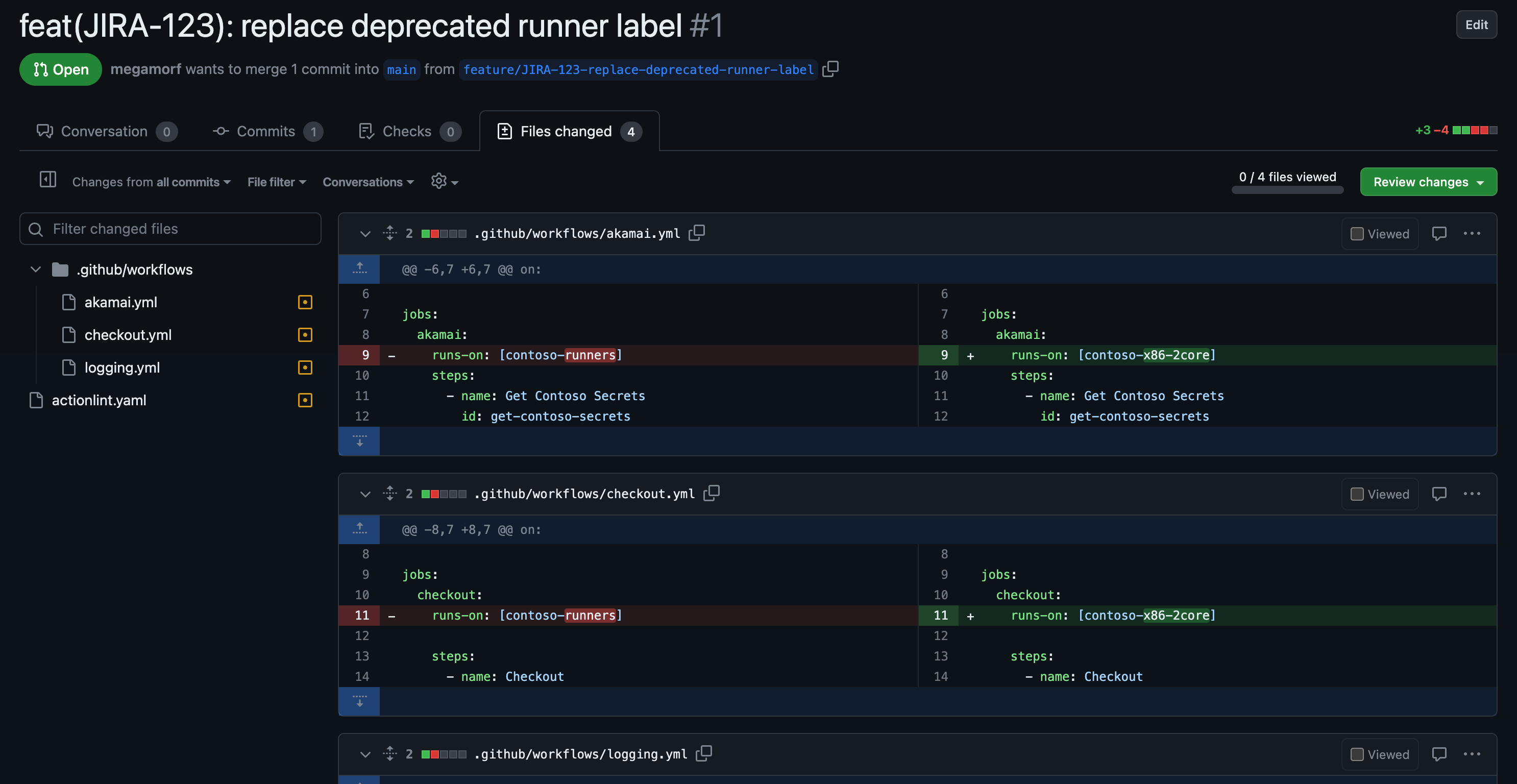
The PRs can now be reviewed:
Merge
There is also a merge subcommand for microplane, that supports the following params but in our case we value the manual aspect of PR reviews:
  -h, --help                     help for merge
      --ignore-build-status      Ignore whether or not builds are passing
      --ignore-review-approval   Ignore whether or not the review has been approved
  -m, --merge-method string      Merge method to use. Possible values include: merge, squash, rebase (default "merge")
  -t, --throttle string          Throttle number of merges, e.g. '30s' means 1 merge per 30 seconds (default "30s")
It also inherits the --repo param from its parent command:
-r, --repo string single repo to operate on
